How to Add Numbers in Excel

[ad_1]
Did you know you can write Python code in a spreadsheet?
You’d be surprised how many different ways there are to do things in Excel. Below, I’ll show you 9 ways to add two or more numbers. You can skip to a certain section if you’d like to see that method:
Video Walkthrough
If you prefer to watch me go through each of these in a demo workbook, here’s a video for that:
To write a formula or a function in Excel (which we’ll be doing in the examples below), start out by simply typing an equals sign in a cell.
=
This triggers Excel to know that what follows will be a formula or a built-in function.
Manual
This is simplest version of a formula in Excel. Start out with the equals sign, and then type in the numbers and operation you want to do. Just like a calculator:
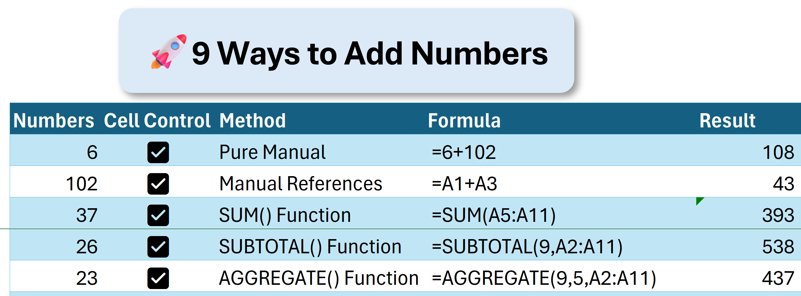
=6+102
Pressing enter will result in 108 being listed in the cell

References
The next step up in Excel is to start using cell references. Notice that on the top and on the left side of the main spreadsheet area, there are columns designated by letters and rows designated by numbers.
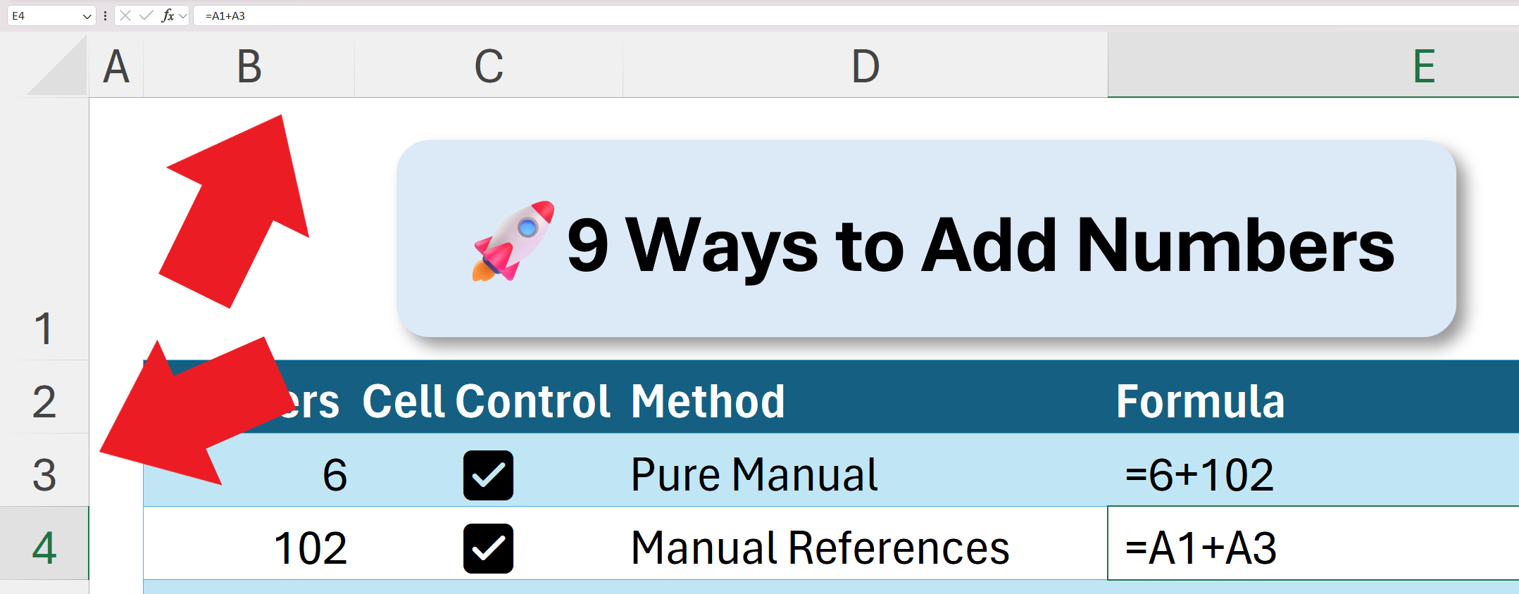
We can refer to specific cells using “A1” notation. Like a set of (x,y) coordinates on a graph, this simply means that by referring to C4, for instance, we are referring to the cell found in column C, row 4.
To add numbers using references, we start again with the equals sign and refer to the values in specific cells directly.
This has the added advantage of being dynamic. If a value is changed in one of the cells, the result of the sum automatically updates.
=SUM(A1+A3) provides us with the value of the numbers in A1 and A3.
SUM()
The first two methods are examples of using formulas. We manually give Excel a series of instructions that it executes.
Excel also has built-in functions which we can use by starting with the equals sign and then referring to the function by name. Functions also take variables which we pass to them by using a set of parenthesis after the name of the function.
The SUM() function takes either a range or a comma-separated list of cell references. It then returns the sum of all the numbers in the range.
You can select a range by either clicking and dragging or by declaring one by typing in the A1 notation with a colon in between the top left cell and the bottom right cell of the range.
SUM(A5:A11) adds all the numbers in cells A5, A6, A7, A8, A9, A10, A11

SUMIF()
A more powerful version of SUM() is the SUMIF() function. This adds conditional logic. It needs at least two variables: a range and a condition. We could give it the same range as above and have a condition be that it only adds up numbers that are greater than zero.
A third, optional variable is a sum_range. This allows for us to match a condition in one range with the sum of values in another range.
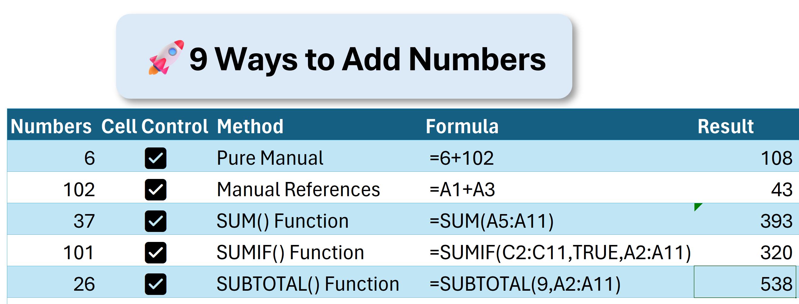
In the example sheet, I have inserted checkboxes in column C. Checkboxes in Excel are a new feature. This is the range that I’m checking for a condition. The condition is TRUE. Now I enter the range that I want to sum if the condition in the corresponding row of the first range is indeed TRUE.
When using a range and a sum_range separately like this, they do have to be of the same size or it will not behave as you want it to.

SUBTOTAL()
Ok, here’s where things start to get interesting.

The SUBTOTAL() function allows us to do a ton of different things. Ultimately, it returns a subtotal of a list or database. But inside of SUBTOTAL() there are other functions. The first argument that we give SUBTOTAL() is a number corresponding to one of these functions:
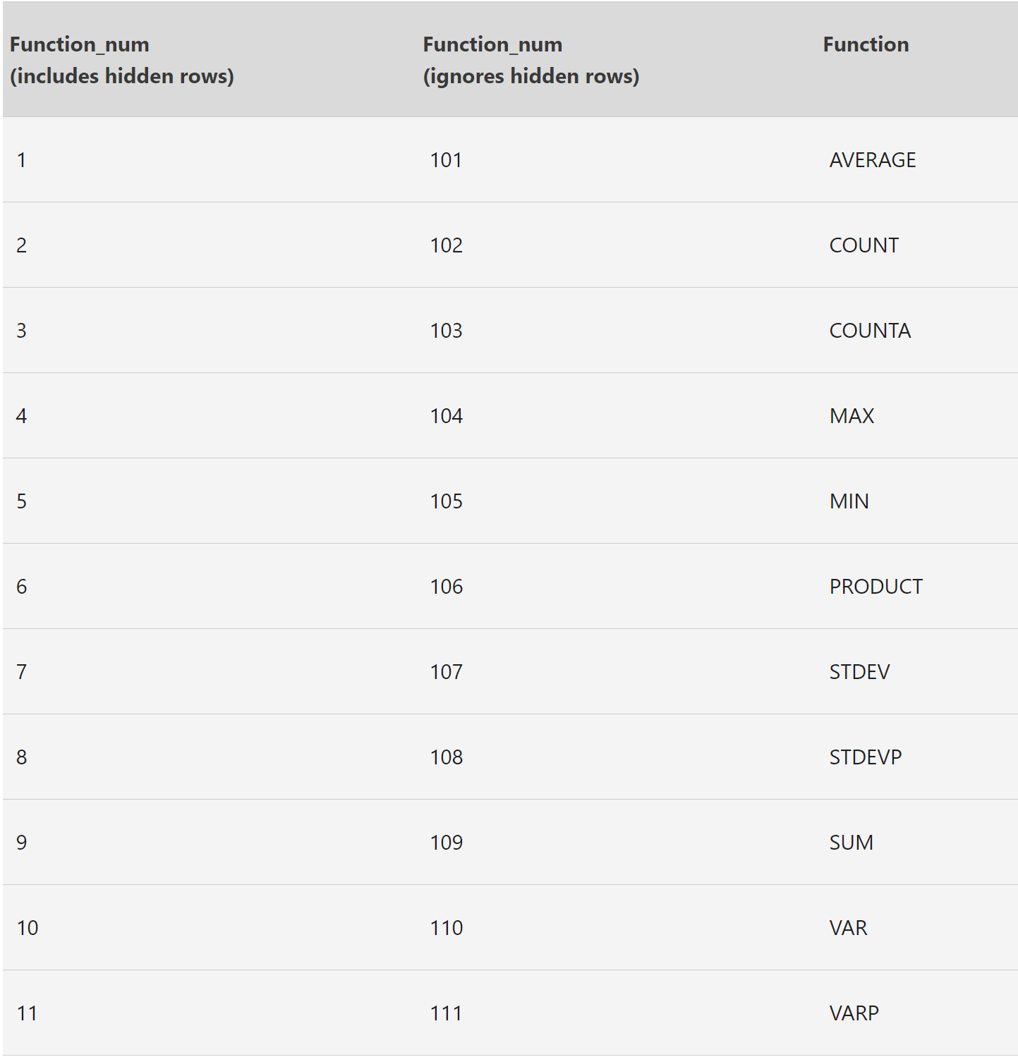
Looking at the function list, we see that 9 or 109 both correspond to the SUM() function which we want to use. If we have hidden rows in our range that we don’t want to include in the sum, we use 109 to ignore those – if not, simply 9.
So the function looks like this: SUBTOTAL(9,B3:B12). This sums B3:B12 even if one or more of those rows are hidden.
AGGREGATE()
We can think of AGGREGATE() as a souped-up version of SUBTOTAL(). It works in the same way but has a lot more built-in functions (19 of them) and allows for detailed specificity on what values, if any, to ignore in the calculation.
AGGREGATE(function_num, options, ref1, [ref2], …) is the full reference formula. Again, we pass it a number corresponding to one of the 19 built-in functions, then an optional argument for what type of values to ignore, followed by the reference array and an optional second reference array.
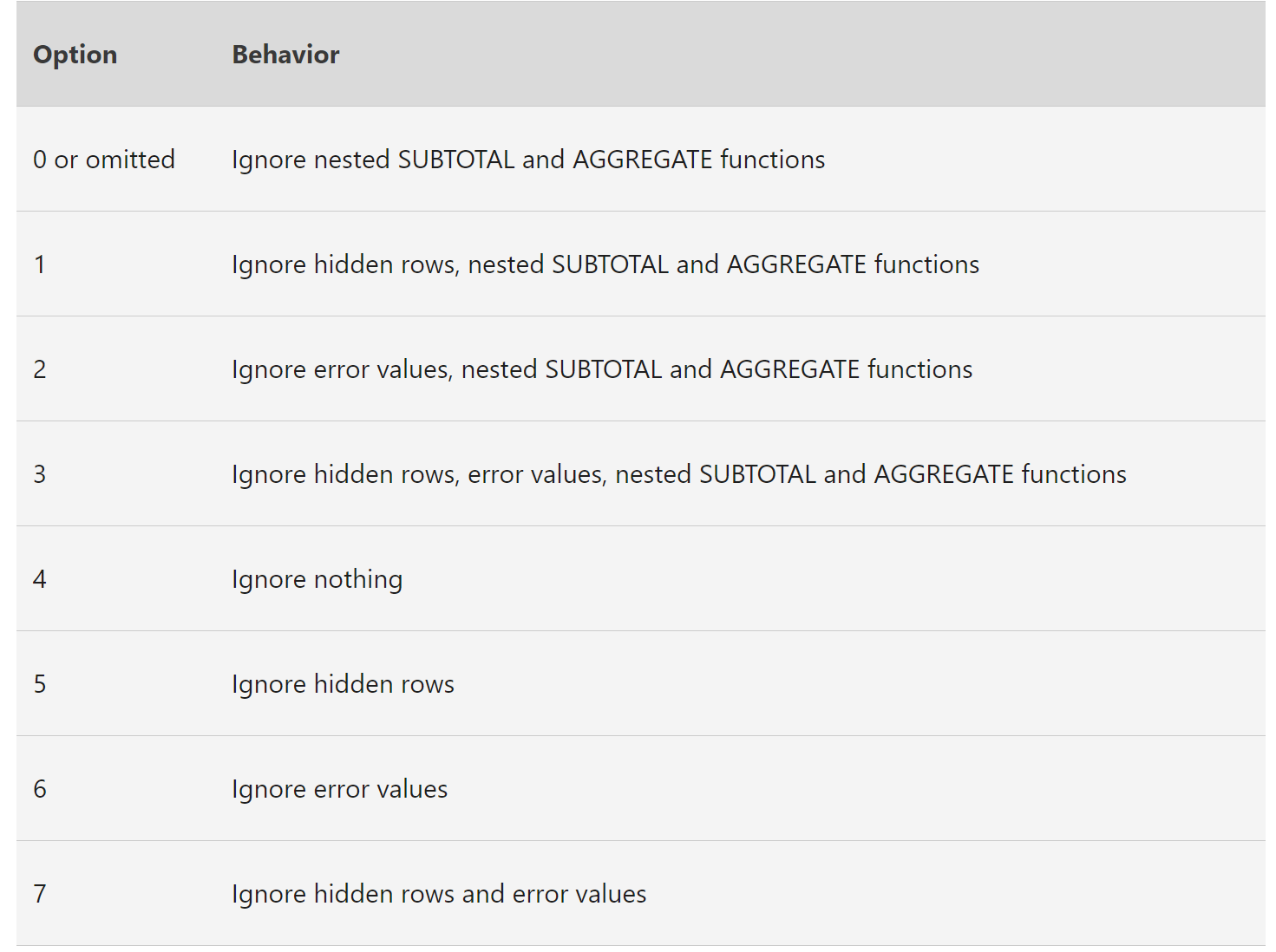
For our example, we again use 9 as our function number, but we can use option 5 to explicitly exclude hidden rows:
VBA
Now we’re warmed up. Let’s get overly complicated.

Visual Basic for Applications is Microsoft’s baked-in programming language in Microsoft Office applications.
Open it up by selecting Visual Basic from the Developer tab.

If you don’t see the developer tab, go to File – Options – Customize Ribbon and add it.
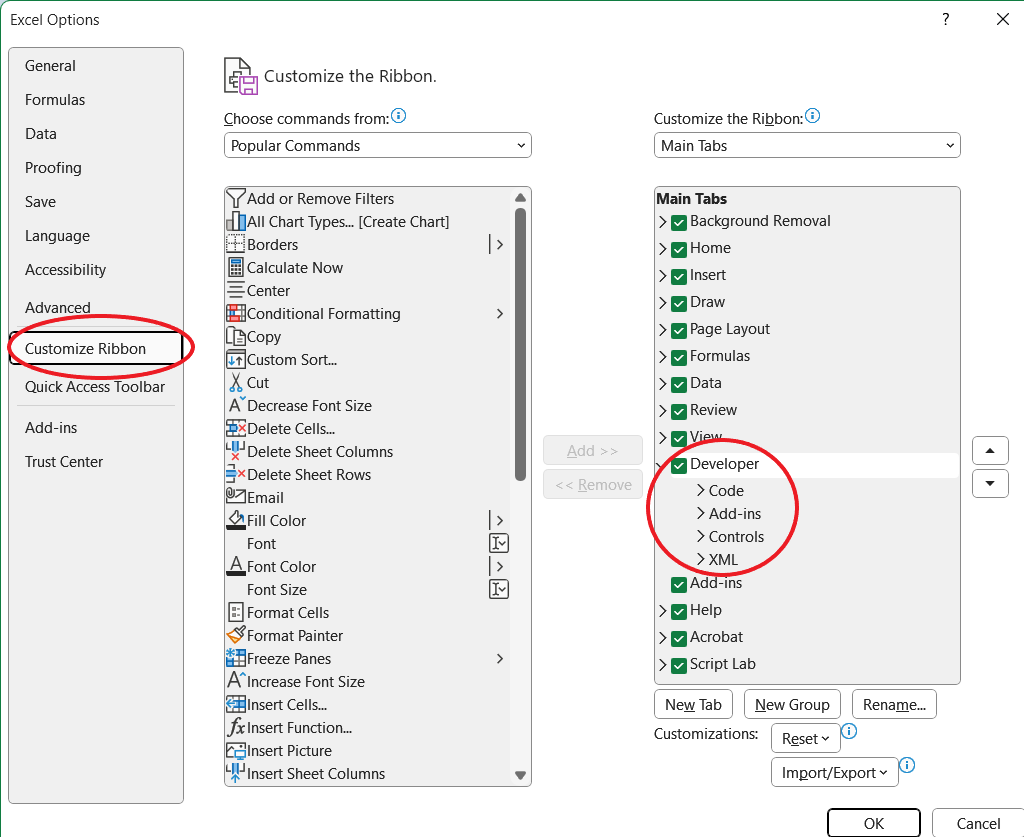
Also, Alt +11 is the keyboard shortcut to open up VBA.
Once here, we can write code to do all sorts of things. Our example isn’t very practical since a function will do it quicker, but the following code will Sum the range A1:A11, put the result in F11 and display a message pop-up with the result:
Sub AssignSumVariable()
   Dim result As Double
   'Assign the variable
   result = WorksheetFunction.Sum(Range("B1:B11"))
   'Show the result
   MsgBox "The total of the ranges is " & result
   'Put the result in cell F9
  Range("F9") = result
End Sub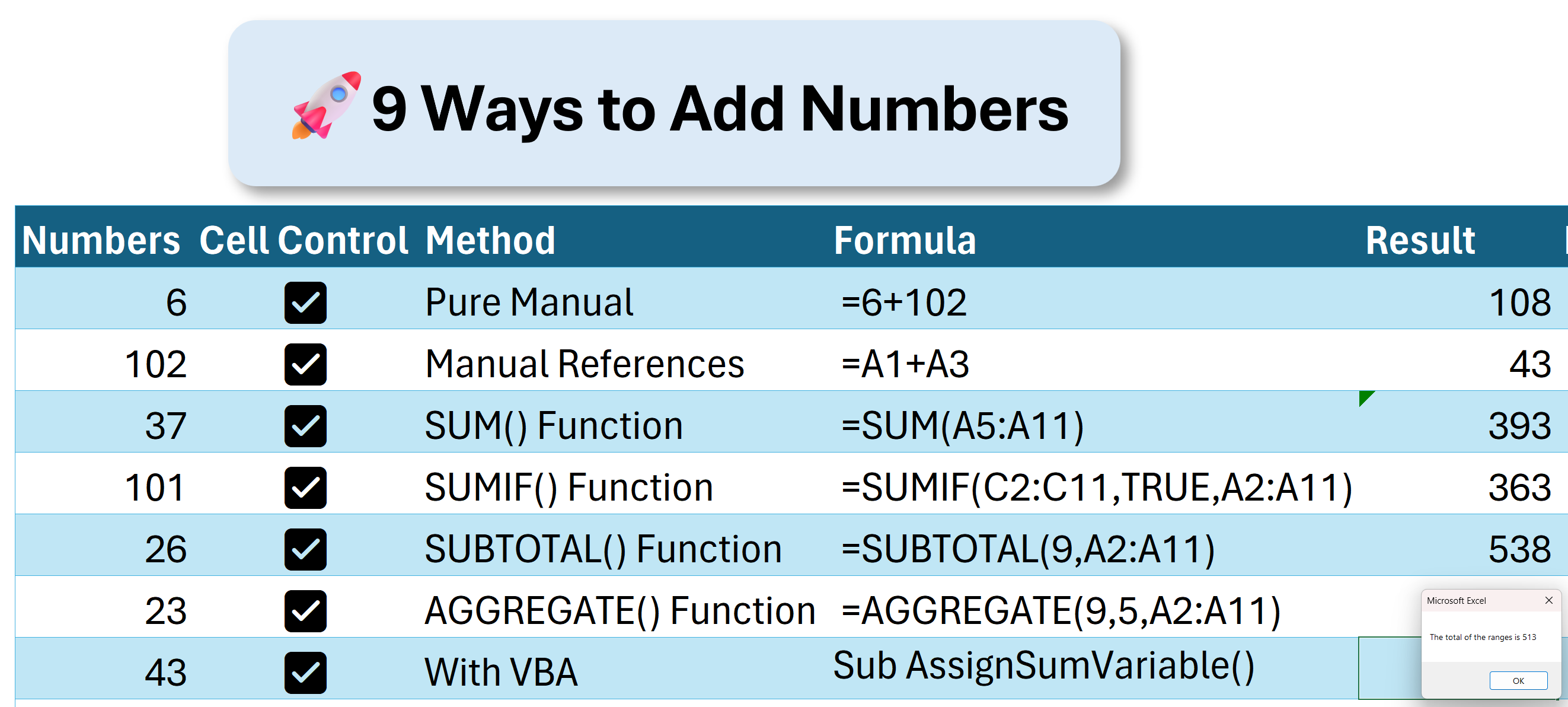
Python
Yes, this is now ridiculous. But, it’s good to know what Excel can do when you have more complicated tasks that require tools like VBA or Python. At the time of this writing, Python is available in Excel for people using the Beta Channel of Excel.

You can check your eligibility and join Microsoft 365 Insider if you want to test out new features like this in the future.
Go to File – Account, and then select the 365 Insider channel button for more info.

Once Python is usable in Excel, you activate it by typing =py and then the tab key. This turns the cell into a Python command line.
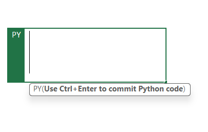
From here, we can write Python code directly in the cell. The following code uses the custom xl() function for Python to use a range. We hold the range in the numbers variable and then using dot notation, we sum that range with the numbers.sum() line:
numbers = xl("'Sum➕'!$B$3:$B$12")
numbers.sum()
Now to execute the Python code, click CTRL + ENTER.
What we now see is that we’ve got a Python Series in the cell:
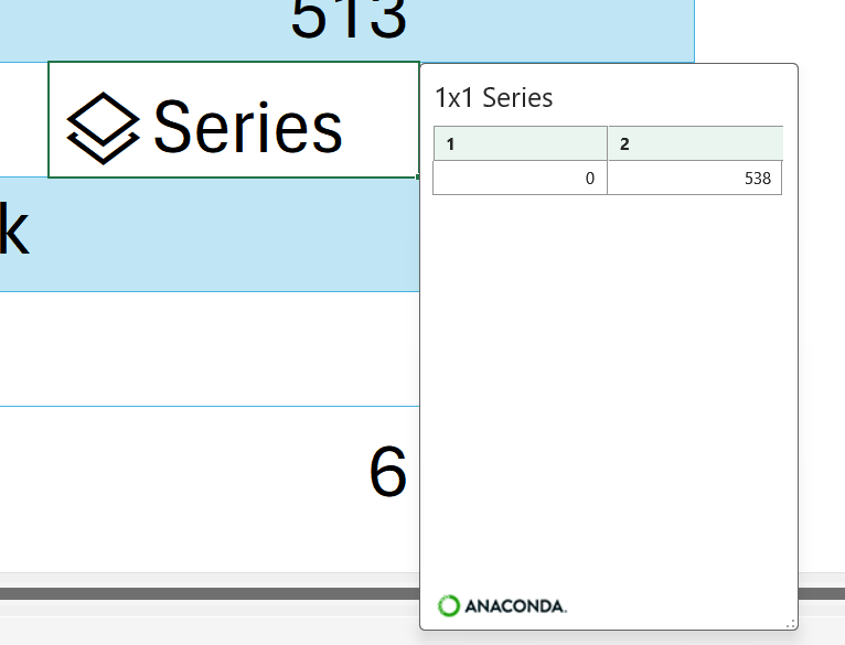
In order to just display the answer, we can click the Python Output selector just to the left of the formula bar and select Excel Value:
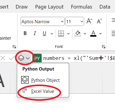
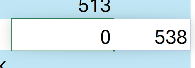
Now, our cell is updated with the correct value.
The real value of Python in Excel comes with manipulating dataframes using built-in libraries like Matplotlib, NumPy, or Pandas.
Okay, take a breath, we’ll finish with something simple and easy…👇
Highlight
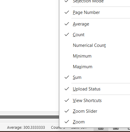
Bonus time. If you highlight cells in Excel by either clicking and dragging mouse over a range, or by CTRL+ Left-Click individual cells, some automatic calculations are visible in the bottom right of the window, including the Average, Count and Sum:
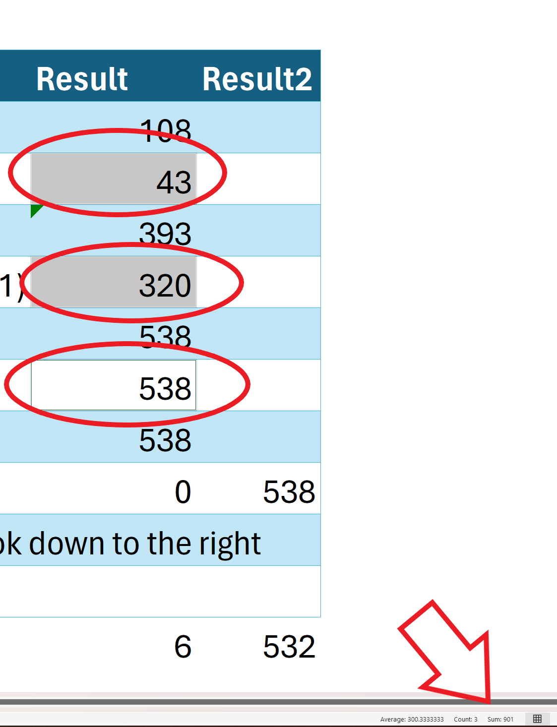
If the sum isn’t immediately visible, right clicking will pull up auto-calculations that you can toggle on and off:
Thanks for reading!
Hope this is helpful for you!
Follow me on LinkedIn: https://www.linkedin.com/in/eamonncottrell/
And YouTube: https://www.youtube.com/@eamonncottrell
Have a great one! 👋
[ad_2]
Source link
